Miniprograms
Introduction
Miniprograms in GraphExpert Professional are “small” Python codes that output a dataset. In essence, a miniprogram is a dataset, except that the source of the data is a program rather than being a set of numbers in the computer’s memory. A miniprogram can be as simple or as complex as the user desires, and the full power of the Python language and add-on modules is available for use. For convenience, GraphExpert Professional provides all of the functions listed in Appendix A: Math Functions in your miniprogram’s namespace for direct use.
Creating a miniprogram
A new miniprogram can be created directly via the Create->Miniprogram main menu choice (or the corresponding toolbar button). The following dialog will then appear:
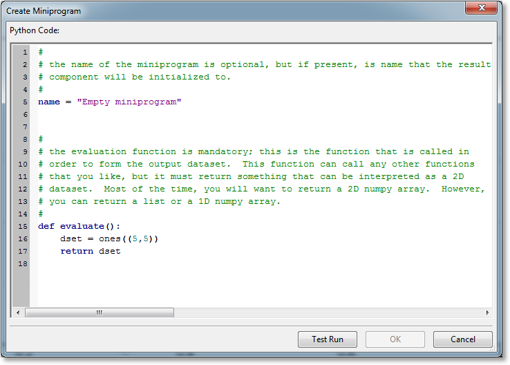
The operation of this dialog is quite straightforward. Enter your miniprogram, and click the Test Run button to test. Once the miniprogram has passed the test, click the OK button.
If the code executes its test run correctly (this does not imply correctness of the code itself), an information bar will appear at the bottom to indicate this, and it will also report the dimension of the returned dataset. If the code does not compile correctly, a stack trace will appear in the information bar to help you track down the problem.
Note
The OK button will not enable until the program has been test run.
Writing the code
Every miniprogram must have one evaluate function. The evaluate function is what will be called whenever GraphExpert Professional determines that the data should be updated.
Rather than trying to reinvent another language for the user to express a model in, GraphExpert Professional uses Python as its base scripting language. Thus, anything that can be done in Python can be done in your miniprograms. This gives the user extreme flexibility, even to do things like download data from a web server that influences the data that the miniprogram returns. Here, your creativity is the only limit.
As you enter the Python code for your function, it is syntax highlighted, and syntax errors are dynamically detected. The standard cut/copy/paste operators are also available for use as you write your code.
Documenting the entire Python language and its capabilities are obviously outside the scope of this document; for this, refer to http://docs.python.org/release/2.6.6. You do not, however, need to be proficient in Python to be reasonably productive creating a miniprogram. Just follow the examples given here and in the miniprogram dialog itself.
Note
Python uses indentation to identify code blocks (for example, the code that should execute when an if statement is true). So, if you have an unexplainable syntax error in your model, make sure that your indentation is correct.
As in regular Python, any characters following a # sign are a comment, and are highlighted in green in the coding window.
Again, every miniprogram must have an evaluate function defined, and furthermore, the evaluate function should take no (mandatory) arguments. Other items that specify metadata (currently, only name), are optional.
name
This is an attribute to define the name of your miniprogram, which is the name that is used for the component that is created for your miniprogram, by default. The type of this attribute is a string, and should be enclosed in quotes.
evaluate()
This is the most important part of your miniprogram; evaluate() is a function that is called whenever a dataset update is required from your miniprogram.
An example of an evaluate function is the following (with comments removed for brevity):
name = "My miniprogram"
def evaluate():
    dset = ones((10,5)) # create a dataset that contains all ones, 10 rows, 5 columns
    return dset
The evaluate function returns anything that can be coerced into a 2D dataset. This can be a float, a list of floats, a list of list of floats, or (most commonly) a numpy array.
Alternatively, a dictionary may also be returned from the miniprogram. This method is used when the user desires to return some metadata about the dataset along with the dataset itself. If a dictionary is returned, it is required to have the dset key, which should have the dataset to return as its value. Metadata currently recognized by GraphExpert Professional is the colnames key, which maps to a list of column names, and the rownames key, which maps to a list of row names. An example of this is below:
name = "My miniprogram"
def evaluate():
    dset = ones((10,3))
    colnames = ["Distance","Velocity","Acceleration"]
    retval = {'dset':dset,'colnames':colnames}
    return retval
Any other Python functions in your script (denoted by the def keyword) other than evaluate are ignored. This means that you can create your own Python functions and call them from your evaluate function as you wish.
Reserved Words
All mathematical functions supported by GraphExpert Professional, such as sin, cos, tan, exp, etc., are also reserved words. See Appendix A: Math Functions for a complete list of the mathematical functions supported.
Miniprogram examples
A simple function
Certainly, the example below is more appropriately implemented via a Function (Create->Function). However, this example is useful to show how simple a miniprogram can be, in order to get you starting using them. This example just computes the sin function between 0 and 2*pi, and returns the dataset:
name = "sin function"

def evaluate():
   n = 101
   x = linspace(0,2*pi,n)
   y = sin(x)
   dset = column_stack((x,y))
   return dset
The “linspace” call creates a vector from 0 to 2*pi, made up of n points; then we take the sine of every entry in that array, returning the result in y. At this point, we have two separate 1D arrays, of dimension 1x101. We would like to return the x data in the first column of a dataset, and the y data as the second column. So, we first “column stack” the two arrays to get a 101x2 2D dataset, Now, just return that dataset, we are are done.
Blasius solution
The following miniprogram calculates the Blasius solution (describes the fluid boundary layer that forms near a flat plate under 2D, laminar, and steady conditions and a uniform oncoming flow) and returns it as a dataset:
import scipy
import scipy.integrate

name = "Blasius Solution"

def blasius(y, eta):
    return [y[1], y[2], -0.5*y[0]*y[2]]

def evaluate():
   n = 201
   initial_condition = [0,0,0.33206]
   eta = linspace(0, 10, n)
   y = scipy.integrate.odeint(blasius, initial_condition, eta)
   eta = eta.reshape((n,1))
   dset = hstack((eta,y))

   colnames = ["eta","y","yp","ypp"]

   return {'dset':dset,'colnames':colnames}
In this example, you can see that the evaluate() function uses the ordinary differential equation solver available in scipy. All of the functionality in scipy is available, which includes numerical integration, optimization, and many other very useful algorithms.
Ellipse
The following miniprogram calculates the points for an ellipse:
name = "Ellipse"

def evaluate():
    a = 2.0 # major axis
    b = 1.0 # minor axis
    x = linspace(-a,+a,201) # create 201 points between -a and +a
    y1 = b*sqrt(1-x**2/a**2) # evaluate the ellipse equation
    dset = vstack((x,y1,-y1)).T # stack the datasets vertically, take transpose

    # the output dataset is 200x3.
    return dset
Moody diagram
The Moody diagram example (see the examples shipped with GraphExpert Professional) demonstrates using a miniprogram in order to solve the Colebrook equation in order to find a family of constant roughness curves. This particular example uses the scipy optimizer in order to do so. Please see the example for further details; you can see each miniprogram by right-clicking on the appropriate component, and choosing Edit Miniprogram.