Managing Datasets and Functions

Introduction

GraphExpert Professional is designed to take raw data as generated by your own process (such as experimental data, raw survey results, etc.), manage and transform that data, and then visualize the data. This chapter focuses on the management and manipulation of these data. To most effectively use the application, an understanding of components is necessary.

What is a Component?

By way of definition, a component is anything that can be visualized in one or more graphs. A dataset is a component that is discrete in nature; a function is a component that is continuous in nature. Both can be managed and manipulated in GraphExpert Professional. Datasets are typically created as documented in Creating new datasets. Functions are created as documented in Functions. In the abstract sense, a component is simply a source of data; either directly as is the case with datasets, or indirectly as is the case with functions (a function must be queried in order to return data).

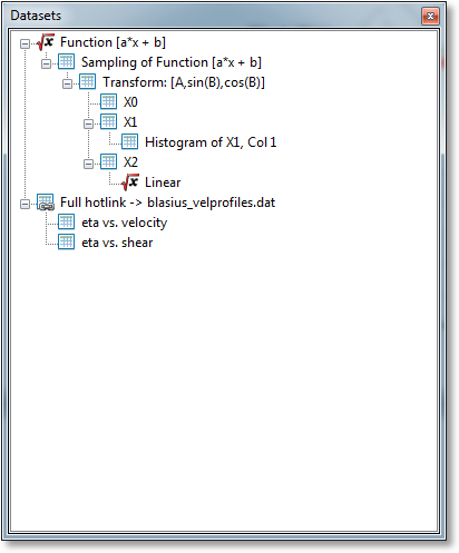
The crux of GraphExpert Professional’s management is that a component (function or dataset) can be derived from another. If this is done, there is then a parent-child relationship between these two components, and the child is automatically updated whenever the parent changes. Any changes in components are also automatically reflected on any graphs that happen to be referring to the changed components.

Hovering the mouse over any component will show an informational tooltip relevant to that particular component.

To move a component up or down (in order to reorder them), select the desired component, hold the Alt key, and press the up/down arrows.

Operations on any component

Details

The details for any component can be queried by right clicking it, and selecting Details from the resulting menu. The details shown are appropriate for the component selected.

Send to current graph

A component can be visualized on the currently visible graph (in the “Graphs” pane) by right clicking it, and selecting Send to current graph. Alternatively, the component can be dragged and dropped onto the visible graph.

Send to new graph

A component can be visualized on a new graph (in the Graphs Pane) by right clicking it, and selecting Send to new graph.

Renaming

Any component can be renamed by right clicking it, and selecting Rename from the resulting menu. Alternatively, the component can be renamed by left clicking on an already-selected component, which makes the name editable in-place. Also, F2 can be pressed to begin the renaming process.

Cloning

Any component can be cloned by right clicking it, and selecting Clone from the resulting menu. Cloning a component creates a copy of it, in its current state, and places the copy at the top level of the component hierarchy (meaning that the clone does not depend on any other component). The clone’s name is the same as the component that it was cloned from with “Copy of” prepended.

If the component being cloned has descendants, these are cloned as well and properly placed as descendants of the clone.

Deletion/Removal

Any component can be removed by right clicking it, and selecting Delete from the resulting menu. If a component is deleted, any graph that is visualizing that component will update appropriately (the series will be removed).

Operations on Datasets

Column split

A dataset can be column split, placing each of its columns into a separate dataset for further manipulation. To perform this, right click a dataset, and select Column split from the resulting menu. This creates ncol new child datasets, where ncol is the number of columns in the dataset selected. Since these new datasets are children, they are noneditable and update automatically when the parent changes.

Split

A dataset with multiple dependent variables can be split, which means to create n new datasets from the marriage of the independent variables with each of the dependent variables separately. For example, if a five-column dataset is present with two independent variables and three dependent variables, then three new child datasets will be created: dataset #1 with the independent variables and dependent variable #1, dataset #2 with the independent variables and dependent variable #2, and dataset #3 with the independent variables and dependent variable #3.

Since these new datasets are children, they are noneditable and update automatically when the parent changes.

Join

Multiple datasets may be joined into one. To join datasets, first shift-select (or ctrl-select) them, right click, and select Join into NxM dataset; N and M will be appropriately filled by the size of the dataset that will be formed from the operation.

GraphExpert Pro automatically detects whether or not the selected datasets are compatible, and in what direction the joining can occur:

• If the selected datasets all have the same number of columns, the Join menu option will indicate that the datasets will be stacked vertically in the joining process. For example, a 10x2 and 15x2 dataset will result in a 25x2 dataset (25 rows and 2 columns).
• If the selected datasets all have the same number of rows, the Join menu option will indicate that the datasets will be stacked horizontally in the joining process. For example, a 10x2 and a 10x3 dataset will results in a 10x5 dataset (10 rows and 5 columns).
• If the selected datasets match in both rows and columns, both joining directions will appear in the context menu, and you will be able to choose the desired joining process.
• If the selected datasets do not have the same number of columns (or rows), the Join context menu option will not be shown at all.

The datasets will be joined in the order that they were selected.

Reclassify

A dataset can have its columns reclassified according their desired use (independent variable, dependent variable, or standard deviation column (see Datasets). To perform this, right click a dataset, and select Reclassify from the resulting menu. See Reclassifying columns for details on how to attain the classification that you desire for your dataset.

If the desire is to rearrange columns, a better tool is the Transform capability, documented below.

Transform

The dataset transformation tool in GraphExpert Professional is a very useful and powerful mechanism that can be used to derive other datasets from one that is present. To access the tool, right click a dataset and select Transform. The following dialog will be presented:

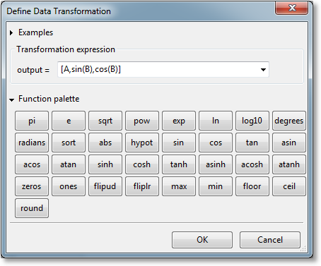
A new expression can be typed directly into the Transformation expression field. Here, the full complement functions as documented in Appendix A: Math Functions can be utilized. For convenience, however, a function palette can be expanded, which appears as a set of calculator-like buttons. Pressing any of these palette buttons will insert the corresponding text into the Transformation expression field, or you are free to type the expression out yourself. Remember that the function palette only has a subset of the available functions in GraphExpert Professional.

A transformation expression is essentially just a list of a columns (more generally, a list of 2D datasets). This list of columns is glued together horizontally in order to form a new dataset. The letters “A”, “B”, “C”, etc. stand for columns of the original dataset (obviously, this limits transformations to dealing with only the first 26 columns of the dataset using this notation; use DSET if it is desired to access more columns; eg., DSET[:,27], which means all rows and the 28th column). The name “DSET” stands for all of the columns of the original dataset.

Slice indexing (e.g., A[5:10], A[-5:], A[0:-1]) can also be used in order to specify a region, as well. Slices are zero based, and the slice runs from the first index up to but not including the last index. With the slicing operators, you can manipulate any subset of the dataset that you like. For example, A[5:10] will extract the 6th through 10th rows of column A. Or, DSET[1:3:5:10] extracts the 6th through 10th rows of columns 1 and 2.

The transpose operator ”.T” may be used to take the transpose of any column, dataset, or section of a dataset. For example, if you want to extract the top left section of a dataset and take the transpose of that, the expression would be [DSET[0:5,0:10].T].

Examples of usage of the transformation dialog are below; these examples range from extremely simple to moderately advanced, to demonstrate the types of transformations that can be accomplished.

In all of these examples, let us assume that the original dataset (the one that we selected when choosing Transform from the context menu) has four columns.

To extract the first column:

[A]

To move the last two columns to the front:

[C,D,A,B]

To create a dataset consisting of the first column and three copies of the last column:

[A,D,D,D]

To keep the first column and apply the sin() function to the second column (discarding the rest):

[A,sin(B)]

To create a new dataset keeping the first column, and adding the other three columns of the original dataset to form the second column:

[A,B+C+D]

To create a new dataset, offsetting column B by a constant to form three new columns:

[A,B+1,B+2,B+3]

To square all entries in the second column:

[A,B^2,C,D]

To raise the elements in column B to the power given by the corresponding elements in column C:

[A,B^C]

To convert column A from degrees to radians, sort B, and reverse the entries in column D, and leave column C alone:

[radians(A),sort(B),C,flipud(D)]

To add on a new column consisting of all fives:

[A,B,C,D,ones_like(A)*5]

To make a copy of the input dataset (same action as [A,B,C,D]):

[DSET]

To prepend column A to the input dataset, creating a 5 column dataset (same action as [A,A,B,C,D]):

[A,DSET]

To create a new dataset with rows 5-10 of columns A and C:

[A[4:10],C[4:10]]

To create a new dataset with first column and last two columns (note that DSET is a 2D array, so it requires two slicing indices):

[A,DSET[:,-2:]]

To take the standard deviation of every column in a dataset (the dataset returned will be a 1x4 array):

[standarddev(DSET)]

To take the average of the last 3 columns of the dataset (the dataset returned will be a 1x3 array:

[average(B),average(C),average(D)]   -- or -- [average(DSET[:,-3:])]

To transpose the entire dataset:

[DSET.T]

To save every 4th row of the entire dataset:

[DSET[::4]]

Also, previous data transformations that have been defined by the user can be accessed via the small down-arrow pulldown at the right end of the Transformation Expression field.

The transformed dataset is a child of the original one, which means that the transformation will be automatically re-executed whenever the parent dataset changes.

In the end, the result of the transformation is a 2D dataset. If the transformation expression that you have entered is “ragged”; meaning that each entry in the list does not have the same number of rows, GraphExpert Professional will zero fill in order to make the number of rows consistent.

Note

The OK button will not enable until the expression given is valid.

Sort

To sort your dataset, right click a dataset component and select Sort from the resulting Operator menu. You will be queried for the column to use as the key when sorting, and then a new child dataset will be created that contains the sorted values. Sorting is vital for correct results when splining, integration, and differencing.

Transpose

To transpose your dataset, right click a dataset component and select Transpose from the resulting Operator menu. Functionally, the transpose operator is identical to doing a Transform with DSET.T as the transformation expression. However, transposing directly with this menu item also has the feature that row names and column names are also flipped, if they are set.

t-test

To perform a t-test for two columns of data, shift-select or control-select the datasets you want to compute a t-test for, right click, and select t-test from the resulting menu. The t-test will be computed, using each column in all of the selected datasets (there should always be exactly two total columns in all of the selected datasets) as a separate, independent, population.

The calculation of the t-test will give you a new top-level component, which holds the t-test calculation results. The t and p value are given. Standard practice is to reject the null hypothesis that the two columns of data were sampled from populations with the same mean, if P < 0.05 (this is for 95% confidence).

Note that t-tests will NOT update as their parents are changed; there is currently no capability within GraphExpert Professional to keep track of multiple parents; for this reason, a top-level, non-updating component is created. If you want to update the t-test due to its parent datasets changing for some reason, it must be recomputed.

ANOVA (Analysis of Variance)

To perform a one-way ANOVA of a list of datasets, shift-select or control-select the dataset components you want compute an ANOVA for, right click, and select ANOVA from the resulting menu. The ANOVA will be computed, using each column in all of the selected datasets as a separate population.

The calculation of the ANOVA will give you a new top-level component, which holds the ANOVA calculation results. The F and p value are given, along with critical F-values for confidences of 85%, 90%, 95%, and 99% respectively. If F < Fcrit, the null hypothesis (that there is no statistical difference between the set of columns) cannot be rejected. Correspondingly, if F > Fcrit, the null hypothesis can be rejected; there is a statistical difference between the set of columns. The P-value is the probability that one or more of the columns are drawn from a different population, and can certainly be used in lieu of comparing F to Fcrit. Standard practice is to reject the null hypothesis that all of the data were sampled from populations with the same mean, if P < 0.05 (this is for 95% confidence).

Note that ANOVAs will NOT update as their parents are changed; there is currently no capability within GraphExpert Professional to keep track of multiple parents; for this reason, a top-level, non-updating component is created. If you want to update the ANOVA due to its parent datasets changing for some reason, it must be recomputed.

Process Replicates

The Process Replicates operator works on a dataset with multiple dependent variables. An average and standard deviation (across the rows) is taken for all dependent variables, Then, the dependent variable columns are replaced with the average and standard deviation columns.

For example, let’s say that your 50x16 dataset consisted of single x (independent varaible) column, and 15 y (dependent variable) columns. Process replicates will take the average and standard deviation across the rows of the 15 dependent variable columns. The 50x3 output dataset then consists of your original x column, the average column, and the standard deviation column.

This operation is common when the dependent variable columns are repeated measurements for the same dependent variable. This functionality allows you to quickly reduce this situation to a data set that has a column for the independent variable, a column for the dependent variable, and a column for the standard deviation in the dependent variable.

Moving Averages

Moving average applies an averaging window to each point in a dataset, in turn, in order to generate a new set of data. The size and type of window determine the amount of averaging that will take place. To calculate a moving average, right click a dataset in the Components pane, and select Moving average from the resulting Operators menu. A dialog will appear that will allow you to select the window to utilize for the averaging.

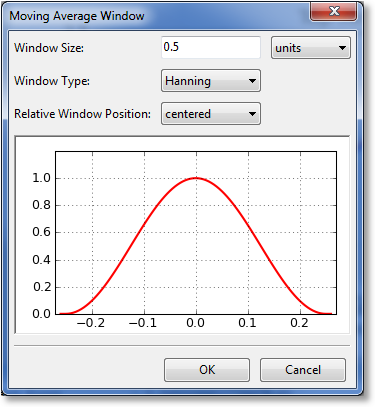
The first parameter to select for the window is its size. Here, you can select the size (sometimes called the extent) of the window in terms of units (meaning a distance along the x axis), or in terms of number of points. The (0.0) location on the preview is always defined to be at the x location of the point being window averaged. The window preview will continually update in order to show the currently defined window. Note that the underlying dataset must be sorted in order for the window to be specified in terms of a number of points. If the dataset is not sorted, the points choice is disabled.

The window type can also be selected from the following:

• rectangular
• Bartlett (triangular)
• Blackman
• Hamming
• Hanning

The window type affects the weighting factor that is applied to each point within the window that is to be averaged. For example, a rectangular window applies a weight of 1 to all points within the window.

Finally, the relative window position can be set. Usually, a centered window is used, which places the center of the window at the same x location as the data point being averaged (location 0.0). Alternatively, you can select a leading or lagging window, which places the window ahead of the data point or behind the data point, respectively.

After tuning the window parameters to the desired settings, click “OK”, and a child component is created in which the moving average is contained.

Compute Differences

The differences of a dataset can be computed by right clicking a dataset component, and selecting Compute differences from the resulting menu. The dependent variable of the resulting dataset is the difference between adjacent rows of the dependent variable of the parent dataset, and the independent variable is the average of adjacent rows of the independent variable of the parent dataset. A new child dataset is created for each differencing operation. As such, the differences are automatically updated whenever the parent’s data is changed.

Differences can be taken for any dataset with a single independent variable. Note that single column datasets have an implied independent variable, which is the row index.

Compute integral

The integral of a dataset can be computed by right clicking a dataset component, and selecting Compute integral from the resulting menu. An integral is computed via Simpson’s rule, using the independent variable vs. each dependent variable in the dataset. Note that the result of an integral operation is a 1x1 dataset. A new child dataset is created for each integral operation. As such, the integrals are automatically updated whenever the parent’s data is changed.

Integrals can be taken for any dataset with a single independent variable. Note that single column datasets have an implied independent variable, which is the row index.

Compute Histogram

A histogram (single column datasets only) can be computed by right clicking a dataset component, and selecting Compute Histogram from the resulting menu. A dialog will appear such that the number of bins in the histogram can be selected.

The resulting dataset contains the bin edges as the independent variable, and the frequency of occurrence as the dependent variable. This dataset is a child of the original dataset, and as such, will update automatically whenever the parent’s data is changed.

Compute DFT

A Discrete Fourier Transform (single column datasets only) can be computed by right clicking a dataset component, and selecting Compute DFT from the resulting menu. The resulting dataset contains the frequency in as the independent variable, and power (which the square of the real and imaginary components of the computed DFT for the data) as the dependent variable. Only the first half of the power spectrum is valid (due to the Nyquist criterion) and therefore only the first half is returned. When the input data has a length that is a power of 2, the Fast Fourier Transform (FFT) algorithm is used to compute the DFT.

This dataset is a child of the original dataset, and as such, will update automatically whenever the parent’s data is changed.

Linear Regression

A linear regression can be computed by right clicking a dataset component, and selecting Linear Regression from the resulting menu. The result of performing the linear regression is the function

where a and b have been adjusted as to optimally fit the data. This function is a child of the dataset, and as such, will update automatically whenever the parent’s data is changed.

Polynomial Regression

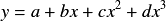
A polynomial regression can be computed by right clicking a dataset component, and selecting Linear Regression from the resulting menu. The result of performing the polynomial regression is the function

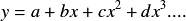
where the parameters a, b, c, etc. have been adjusted as to optimally fit the data. This function is a child of the dataset, and as such, will update automatically whenever the parent’s data is changed.

Upon choosing a polynomial regression, the following dialog is presented:

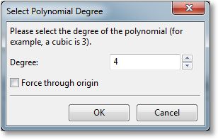
Here, the degree of the polynomial regression (up to 19th degree polynomials are supported) can be selected, and the user can choose whether to force the polynomial through the origin; in that case, the constant a (the intercept) is always zero, and only the other parameters are optimized.

This function is a child of the dataset, and as such, will update automatically whenever the parent’s data is changed.

Cubic Spline

A cubic spline can be computed by right clicking a dataset component, and selecting Cubic Spline from the resulting menu. The result of performing the cubic spline is a function made up of piecewise cubics

that are continuous at the knots, as well as the first two derivatives being continuous at the knots. Note that the spline computed is a natural cubic spline, which means that 2nd derivative is zero at the endpoints.

This function is a child of the dataset, and as such, will update automatically whenever the parent’s data is changed.

Operations on Functions

Edit Function

Selecting Edit Function will allow you to edit the expression (for Simple functions) or Python code (for Programmed functions), the parameters, and the default domain for a function.

Sample

Sampling gives the ability to create a dataset from a continuous function. A 2D or 3D function can be sampled by right clicking it, and then selecting Sampling from the resulting menu. The following dialog will be shown:

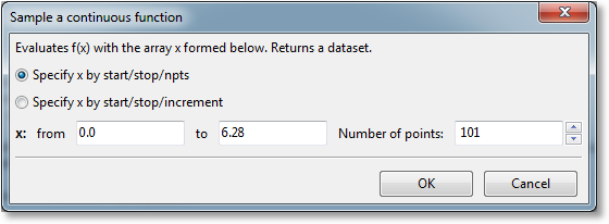
The sampling can be specified by either giving the start and stop point along with the desired number of points (samples), or one can give the start and stop point along with the distance (increment) between each sample. Upon pressing OK, the new dataset is created. This new dataset is a child of the function, and as such, will update automatically whenever the parent is changed (for functions, this typically means that the function parameters are changed in some way).

For a 3D function, a similar sampling dialog will appear, but allows the user to sample in the two independent variable directions.

Compute Derivative

The derivative of the function at a particular point can be computed by right clicking a function component, and selecting Compute derivative from the resulting menu. The derivative is computed via finite difference, and the result is a new dataset component that contains the result. A new child dataset created for for the derivative; as such, the derivative is automatically updated whenever the parent function is updated.

Derivatives can be taken for any function with a single independent variable.

Compute integral

The integral of a function can be computed by right clicking a dataset component, and selecting Compute integral from the resulting menu. A dialog will appear to allow you to type in the limits of integration. An integral is then computed, with the output being a 1x1 dataset. A new child dataset is created for each integral operation; as such, the integral is automatically updated whenever the parent function is updated.

An integral can be taken for any continuous function with a single independent variable.